How to partially rasterize a figure plotted with R

If you work with datasets that are big enough in R you will eventually encounter situations where your plots are so complex that they do things like crash Preview.app on macOS. For me this happens a lot when I generate huge scatterplots with very dense overplotting. These don’t add much information to the figure but nevertheless must be rendered by your PDF viewer, slowing it down and generally making a mess of things.

I recently encountered a situation where a journal’s editing office couldn’t handle a particularly complex figure and requested that the figure be converted into a raster format. This is less than ideal compared to a vector format like PDF: you can’t do things like select text from a rasterized PNG and it’s generally just less usable. (More info on raster vs. vector images). Would it be possible to convert the complex parts of the figure to a raster format while keeping everything else vectorized?

The answer is yes! And it can all be done in R, with no fiddly conversions by hand and trying to place things precisely in Illustrator.

Let’s use the built-in mtcars dataset to as an example, and include some colors and a legend:

plot(mpg ~ wt, data = mtcars, col = factor(mtcars$cyl), pch = 19)
legend(x = 5, y = 34, legend = levels(factor(mtcars$cyl)), col = c(1:3), pch = 19)

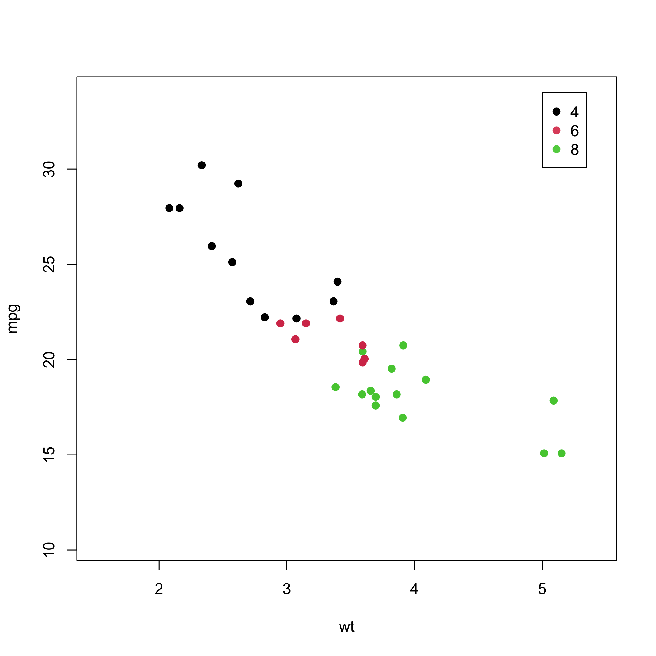
Note that the legend overlaps the plot area. If you were to simply plot the entire thing as a PNG and then crop out the plot area, you’d either also have to rasterize the legend (and lose the ability to edit the text in Illustrator later) or manually erase the legend (let’s avoid doing things by hand).

Let’s modify this code step by step. First set up our PDF device, with an output size of 7 by 7 inches.

pdf("mtcars.pdf", width = 7, height = 7)

Next set up the plot axes and legend. These are the same plot commands as before, but here type = "n" is specified, so that only the axes are set up, but no data are actually plotted.

plot(mpg ~ wt, data = mtcars, col = factor(mtcars$cyl), type = "n")
legend(x = 5, y = 34, legend = levels(factor(mtcars$cyl)), col = c(1:3), pch = 19)

Now we must figure out how big our plot area actually is. To do so, use the par function to extract the plot limits. This returns a 4-element vector, where the first two elements are the x-coordinates and the last two elements are the y-coordinates of the plot area.

coords <- par("usr")
# [1] 4.156 8.044 0.764 7.136

However, these coordinates are in “user” space, meaning that they don’t correspond to the physical dimensions in the plot device. Use the grconvert functions to convert from user space to plot device space, in inches:

gx <- grconvertX(coords[1:2], "user", "inches")
# [1] 0.82 6.58

gy <- grconvertY(coords[3:4], "user", "inches")
# [1] 1.02 6.18

width <- max(gx) - min(gx)
# [1] 5.76

height <- max(gy) - min(gy)
# [1] 5.16

Now set up a raster device with the dimensions computed from the vector (PDF) device. Note that the PDF device is still active at this point.

png("mtcars_panel.png", width = width, height = height, units = "in", res = 300, bg = "transparent")

Since the plot axes are handled in the vector device, it’s unnecessary to set those up. So avoid the high level plot commands and instead set up the plot areas from scratch. plot.window needs the x and y limits computed earlier, but by default R will expand the limits so that a data point right on the edge of the specified limits doesn’t get cut off.

Tell R to turn off this feature by setting xaxs and yaxs to "i". Also turn off the plot margins with mar = c(0,0,0,0) since that will just be empty space.

plot.new()
plot.window(coords[1:2], coords[3:4], mar = c(0,0,0,0), xaxs = "i", yaxs = "i")

Finally, plot the data points as before and close the PNG device.

points(mpg ~ wt, data = mtcars, col = factor(mtcars$cyl), pch = 19)
dev.off()
# pdf
#   2

Now there are two figures that look like this, one PDF and one PNG:

To combine these, read in the generated PNG file using the png library, and then plot it using the rasterImage function. The relevant code looks like this:

library(png)
panel <- readPNG("mtcars_panel.png")
rasterImage(panel, coords[1], coords[3], coords[2], coords[4])

Note that the coordinates for rasterImage be specified a different order than for the plot.window function from before.

Wrap up by closing the PDF device.

dev.off()
# null device 
#           1 

All together, here is the entire script. It’s a bit different from what’s written above; in particular, I save the rasterized plot area to a temporary file to avoid cluttering up our working directory.

library(png)

pdf("mtcars.pdf", width = 7, height = 7)

# Set up plot axes and legend
plot(mpg ~ wt, data = mtcars, col = factor(mtcars$cyl), type = "n")
legend(x = 5, y = 34, legend = levels(factor(mtcars$cyl)), col = c(1:3), pch = 19)

# Extract plot area in both user and physical coordinates
coords <- par("usr")
gx <- grconvertX(coords[1:2], "user", "inches")
gy <- grconvertY(coords[3:4], "user", "inches")
width <- max(gx) - min(gx)
height <- max(gy) - min(gy)

# Get a temporary file name for our rasterized plot area
tmp <- tempfile()

# Can increase resolution from 300 if higher quality is desired.
png(tmp, width = width, height = height, units = "in", res = 300, bg = "transparent")
plot.new()
plot.window(coords[1:2], coords[3:4], mar = c(0,0,0,0), xaxs = "i", yaxs = "i")
points(mpg ~ wt, data = mtcars, col = factor(mtcars$cyl), pch = 19)
dev.off()

# Windows users may have trouble with transparent plot backgrounds; if this is the case,
# set bg = "white" above and move the legend plot command below the raster plot command.
panel <- readPNG(tmp)
rasterImage(panel, coords[1], coords[3], coords[2], coords[4])

dev.off()

Exercises

1. What would you need to change to plot a different type of data, e.g., a line plot or a 3D plot?
2. How would you apply this to a multi-panel figure?
3. How might this be accomplished with ggplot2 graphics? (Hint: annotation_raster, theme_void)

Postscript

An alternative way to do this would be to write to a null device and use dev.capture to rasterize and copy the the figure to the active device. However, that approach doesn’t appear to work consistently across platforms and devices, so I’ve taken the more portable approach presented here.